hubble_constant

The Hubble constant from the binary-black-hole mass spectrum (spectral siren), with icarogw [57] and bilby [58]/dynesty [60]. The method, its validation and its results are explained in Hubble constant (spectral siren); this page is about running it.

The default setup reproduces the spectral-siren measurements of the GWTC-4.0 cosmology paper [29] (published version v3): H₀ = 105.5 (+46.4 / −35.8) km/s/Mpc with the Power Law + Peak mass model (--mass-model plp, the default) and 72.3 (+42.5 / −25.6) km/s/Mpc with the Multi Peak model (--mass-model mltp). Use one work directory per mass model.

# prepare in the gwtc_analysis environment, then 4 runs, 2 at a time with 2 processes each, and the report
gwtc_analysis hubble_constant --stages prepare
gwtc_analysis hubble_constant --stages sample combine report \
    --icarogw-python ~/.conda/envs/icarogw/bin/python --seeds 1 2 3 4 --parallel 2 --npool 2

Stages

The work is split into stages (--stages, all by default) sharing a work directory (--workdir):

Stage	Does	Needs	Cost
prepare	selects the events, downloads their PE files (restartable; only the extracted samples are kept in --pe-cache unless --keep-pe-files), prepares the injections → inputs.h5, events.tsv	gwtc_analysis environment	~35 GB of downloads the first time
sample	with --inj-fraction auto, first a probe that chooses the injection subset (probe.json, plan.json); then one dynesty run per --seeds value, --parallel of them at a time (logs in <workdir>/logs); resumable from its checkpoint	icarogw	a few minutes of probe, then hours per run
combine	merges the runs → posterior.tsv, corner.png, summary.json, with the numerical-stability diagnostics	icarogw	minutes
reweight	when the runs used a subset of the injections, reweights their posterior to all of them → posterior_reweighted.tsv, weights and effective sample size in summary.json	icarogw	minutes to an hour, in --parallel × --npool chunks
report	--out-report (HTML) and --out-summary (TSV of the posterior quantiles)	gwtc_analysis environment	seconds

Event and injection selection

Option	Default	Meaning
--catalogs	all the runs of the release	catalog keys (GWTC-1 … GWTC-5, or ALL): events and injections restricted to their observing runs (GWTC-1: O1–O2, GWTC-2.1: O3a, GWTC-3: O3b, GWTC-4: O4a, GWTC-5: O4b). The published comparison is shown only for the release's own selection
--sensitivity-release	gwtc4	injections and matching catalogs and runs: gwtc4 = O1–O4a (validated against the paper [29]), gwtc5 = O1–O4b (not yet validated against a published result)
--far-threshold	0.25 per year	events (published FARs, rounded, compared inclusively: FAR ≤ threshold), and real injections (full precision, FAR < threshold), below this false-alarm rate
--snr-threshold	10	semi-analytic O1+O2 injections above this network SNR
--min-mass	3 M☉	both source-frame masses above it: potential neutron stars are left out
--inj-fraction	auto	injections used by the sampler runs: auto (the probe chooses the fastest reliable subset, then the posterior is reweighted to all the injections) or a fraction in (0, 1] (1 = all, as in the paper)
--min-ess-fraction	0.5	smallest predicted effective-sample-size fraction of the reweighting accepted by auto
--reweight-pe-samples	as the runs	PE samples per event of the reweighting target
--mass-model	plp	BBH primary-mass model: plp (Power Law + Peak, Table 3 of the paper) or mltp (Multi Peak: power law and two Gaussian peaks, Table 4)
--exclude	GW231123_135430, GW200105_162426	as in the GWTC-4.0 cosmology analysis [29]

icarogw

gwtc_analysis/h0_icarogw.py is a driver of icarogw, not a modified copy: icarogw is used as installed, through its public API. The LVK also uses a second code, gwcosmo; the two are compared in icarogw and gwcosmo.

• icarogw provides the hierarchical likelihood (PE and injection reweighting, selection term, scale-free rate marginalisation, effective-sample-size checks), the population models (massprior_PowerLawPeak with the m1m2_conditioned_lowpass smoothing, rateevolution_Madau, FlatLambdaCDM_wrap, combined by CBC_vanilla_rate), and the detector-frame conversion for each trial H₀.
• The driver reads inputs.h5 into icarogw's posterior_samples and injections objects, chooses the model components and the priors (Tables 3 and 6 of the paper [29]), runs bilby/dynesty, merges the runs and computes the diagnostics with icarogw's own methods.
• The analysis choices made here, outside icarogw, are the input preparation in hubble_constant.py (event selection, PE distance prior read from each file, injection draw density carried to the detector frame with the spin part divided out and the mixture weights applied) and three settings: at least 10 effective PE samples per event (the paper's choice; the default of icarogw's likelihood class is 20), at least 4 × N_events effective injections (icarogw's default), and the injection subset of the runs, corrected by the reweighting stage.

Only sample and combine need icarogw, which requires Python ≥ 3.12 and usually has its own environment (Installation). Its interpreter is passed with --icarogw-python; the default is the interpreter running gwtc_analysis, and the mode stops before sampling if icarogw or bilby cannot be imported there. The stages run h0_icarogw.py with it, in CPU mode (a config.py with CUPY=False in the work directory) and with the environment's lib/ on LD_LIBRARY_PATH.

Injection subsets, probe and reweighting

Each likelihood evaluation sums over the found injections: with all of them (about one million) it takes about 1.3 s, with 10% about 0.3 s. Sampling with a subset is therefore much faster, but it tilts the posterior: for PLP, 10% of the injections shift H₀ by about +13 km/s/Mpc (0.35σ) (details). The mode keeps the speed and removes the shift in two steps:

1. Probe (before sampling, 5 to 20 minutes). A short ensemble MCMC (emcee, 300 steps), started from prior points with a finite likelihood and using the smallest subset, moves to the region the runs will explore. At its final positions the probe measures, for each subset (10%, 20%, 50%), the time per likelihood evaluation, the scatter σ of ln L_subset − ln L_all, which predicts the effective-sample-size fraction of a reweighting, exp(−σ²), and the fraction of positions that the subset rejects while all the injections accept them (a reweighting cannot recover regions the runs never visit). The rule: the smallest subset at least 1.25 times faster, with a predicted fraction ≥ --min-ess-fraction and at most 5% of rejected positions; otherwise all the injections.
2. Reweighting (after combine). Each posterior sample θᵢ gets the weight exp[ln L_all(θᵢ) − ln L_runs(θᵢ)]. The weighted samples describe the posterior with all the injections; posterior_reweighted.tsv is a resample of them, and the report leads with it. The stage checks that it reproduces the ln L stored by the runs, and reports the effective sample size (Σw)²/Σw² and the samples the full likelihood rejects. A small effective sample size (below ~10%) means the subset was too inaccurate: sample again with --inj-fraction 1.

Validation on the PLP reproduction:

	Predicted ESS fraction, 10% subset	Speed-up per evaluation
probe with prior points only	0.20 (would choose 50%)	1.7× (50%)
probe with the pilot MCMC	0.74 (chooses 10%)	4.7×
measured on the real posterior	0.72

The reweighting stage reproduces the result computed independently: H₀ = 106.5 (+45.0 / −34.0) with all the injections, effective sample size 2564 of 3582. For MLTP it gives 78.5 (+38.7 / −26.7), from 89.1 with the subset, effective sample size 2592 of 3862. The runner's reweight --target-inputs also reweights to a likelihood with other inputs: adding the 137th event of the paper (GW191127) this way gives 105.8 (+44.7 / −33.2) for PLP and 78.6 (+38.0 / −26.5) for MLTP, with effective sample sizes of 68% and 66%. A numeric --inj-fraction bypasses the probe; --inj-fraction 1 samples with all the injections, as the paper does, and needs no reweighting.

Seeds

Each seed is an independent dynesty run (result/<model>_seed<N>_result.json, with <model> = plp or mltp); combine merges all the finished ones, weighted by their evidence.

• All runs sample the same likelihood. The PE samples are shuffled once in prepare, and the injection subset is drawn with a fixed seed. run_settings.json refuses runs with another --mass-model, --nlive, --pe-samples or --inj-fraction values in the same work directory.
• Restarting is safe. Launching again resumes the interrupted runs from their checkpoint and skips the finished ones.
• One process per seed. A lock file (result/<model>_seed<N>.lock, holding the host and process ID) prevents a seed from running twice at once; a lock left by a process that died on the same host is taken over.
• Interrupting the launcher (Ctrl-C) stops its runs after they write their checkpoint.

How many seeds?

The seeds do not change the physics: they set how precisely the sampler describes the posterior.

1. Checking that the runs agree (at least 2 seeds). The evidences ln Z of the runs should agree within their quoted errors (about 0.4), and so should their H₀ intervals. Runs that disagree beyond their errors are not fixed by more seeds but by more live points (--nlive).
2. Precision of the quoted numbers. One run of 100 live points gives about 560 posterior samples, so its median wanders. In the 10 runs of the reproduction, the per-run H₀ medians range from 111.7 to 126.1 km/s/Mpc (standard deviation 4.8), and the ln Z values have a standard deviation of 0.32, consistent with their errors. Combining N runs divides the scatter by about √N:

Seeds (100 live points)	Uncertainty on the H₀ median	Relative to the posterior width (±40)
1	±4.8 km/s/Mpc	12%
4	±2.4 km/s/Mpc	6%
10	±1.5 km/s/Mpc	4%

The PLP posterior is broad, so 3–5 seeds give the result to two significant digits; 10 seeds allow a comparison with a published value at the level of a few km/s/Mpc. The error is a fixed fraction of the posterior width, so the same numbers of seeds hold for narrower posteriors. Fewer runs with more live points are equivalent: 10 runs of 100 live points give about as many samples as one run of about 1000; small runs can be spread over machines and interrupted, but each explores less carefully, which makes the agreement check more important.

Purpose	Settings
Quick look	2 seeds
Result to report	4–5 seeds, or 2 seeds with --nlive 500
Precise comparison with a paper	about 10 seeds

The individual runs of the reproduction:

Seed	Samples	H₀ median	90% interval	ln Z
1	559	118.3	57.6 – 187.5	−3824.59
2	503	126.1	66.8 – 185.3	−3823.65
3	611	123.9	62.2 – 187.8	−3824.66
4	524	112.8	58.8 – 184.2	−3824.02
5	595	111.7	60.2 – 184.3	−3823.71
6	563	119.8	66.6 – 187.1	−3824.30
7	603	115.2	62.9 – 186.7	−3824.13
8	581	123.8	61.3 – 186.9	−3824.21
9	507	120.1	63.0 – 188.8	−3824.22
10	584	118.5	64.7 – 186.4	−3824.09

--npool and --parallel

Nearly all the time of a run goes into likelihood evaluations. At each iteration dynesty replaces the live point of lowest likelihood L_min by a new point with L > L_min, found by a random walk from another live point (about --naccept accepted steps, one likelihood evaluation per step).

              ┌─ worker 1: walk ... → new point A ─┐
 main process ├─ worker 2: walk ... → new point B ─┤ → A replaces the worst point,
 (dynesty)    ├─ worker 3: walk ... → new point C ─┤   B the next worst, ...
              └─ worker 4: walk ... → new point D ─┘

With --npool N, bilby starts N worker processes, each holding a copy of the likelihood, and dynesty runs N walks at the same time. The walks all start from the same L_min, so some of their points are no longer good enough when used: N workers give less than N times the speed.

Option	Parallelises	Effect
--npool	within one seed	each run finishes sooner, with the same result
--parallel	across seeds	more runs at the same time

The machine runs --parallel × --npool processes, which should not exceed its number of CPUs (the mode warns), and each of them holds the likelihood data in memory. For the same CPUs, several seeds with few workers each use the machine better than one seed with many workers.

Machine	Suggested settings
4 CPUs, 8 GB (laptop)	--parallel 1 --npool 4, or --parallel 2 --npool 2 if memory allows
8 CPUs, 16 GB	--parallel 2 --npool 4

Running on other machines

Runs can be spread over several machines that share the work directory: start python gwtc_analysis/h0_icarogw.py run --workdir DIR --seed N with the icarogw interpreter on each, then run the combine and report stages once. The seed locks protect against starting the same seed twice.

Without icarogw on the local machine. h0_icarogw.py only needs numpy, h5py, icarogw and bilby, so the sampling can run on another machine that has icarogw (a computing cluster, for instance):

1. locally: hubble_constant --stages prepare --workdir DIR, then copy DIR/inputs.h5 (about 45 MB) and gwtc_analysis/h0_icarogw.py to a work directory on the remote machine;
2. remotely, with the icarogw interpreter (and LD_LIBRARY_PATH=<env>/lib if needed): python h0_icarogw.py run --workdir RDIR --seed N for each seed, then python h0_icarogw.py combine --workdir RDIR;
3. locally: copy RDIR/summary.json, RDIR/posterior.tsv and RDIR/corner.png (a few MB) back into DIR, which still holds events.tsv, and run hubble_constant --stages report --workdir DIR.

Diagnostics

combine evaluates, over 200 posterior draws, the effective number of injections and the smallest per-event effective number of PE samples, against icarogw's thresholds, and names the events with the fewest. The report flags values below the thresholds; more --pe-samples or a larger --inj-fraction then make the Monte Carlo sums more reliable. On the reproduction, the effective number of injections stayed above 3 800 (threshold 544), while the smallest per-event value had a median of 27 and reached 8 at some draws (threshold 10), for the lightest BBHs such as GW190924.

Example

gwtc_analysis hubble_constant --stages prepare
gwtc_analysis hubble_constant --stages sample combine reweight report \
    --icarogw-python ~/.conda/envs/icarogw/bin/python --seeds 1 2 3 4 --parallel 2 --npool 2

The report leads with the H₀ posterior, compared with the published value of the same mass model:

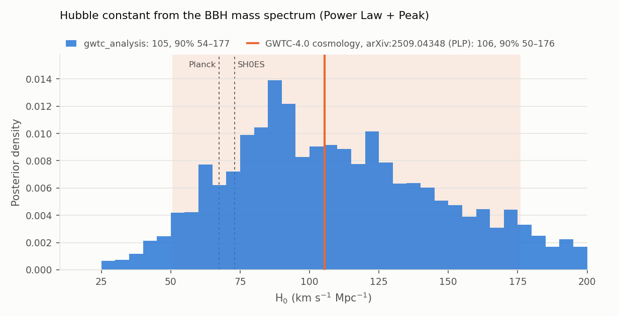
GWTC-4.0, Power Law + Peak: 10 runs with 10% of the injections, reweighted to all of them; the published result (orange line, 90% band) and the Planck and SH0ES values for comparison. Details in Hubble constant (spectral siren).

All options: CLI reference.