Merger rates

How many compact-binary mergers happen per unit volume and time? The rates mode answers with the simplest estimator that corrects for selection effects: a count divided by a sensitive volume-time. Usage: rates.

The estimator

Detections form a Poisson process. For a population with a rate density \(R\) (per Gpc³ per year of source-frame time), the expected number of detections is

\[ N_\text{exp} = R\, \langle VT \rangle , \]

where \(\langle VT \rangle\) is the sensitive volume-time of that population, computed from the injections. With \(N\) detections, the likelihood is \(p(N \mid R) \propto (R\langle VT\rangle)^N e^{-R\langle VT\rangle}\). With the Jeffreys prior \(p(R) \propto R^{-1/2}\), the posterior of the rate is a Gamma distribution:

\[ R\,\langle VT \rangle \sim \text{Gamma}\!\left(N + \tfrac{1}{2},\, 1\right), \]

and the quoted median and 90% interval are its quantiles divided by \(\langle VT \rangle\). The interval is purely statistical (Poisson): the population shape is fixed.

Populations

The events are classified by their median source-frame masses, neutron stars being below 2.5 M☉:

Class	Condition
BNS	both masses < 2.5 M☉
NSBH	secondary < 2.5 M☉ ≤ primary
BBH	both masses ≥ 2.5 M☉

Each class has a fixed population model, used to compute its ⟨VT⟩ (table). The BBH model is the GWTC-3 Power Law + Peak (Talbot & Thrane 2018 [15]; parameters of GWTC-3 population [12]): a power law in the primary mass with a Gaussian peak near 34 M☉ and a smooth low-mass turn-on.

The BBH rate is reported two ways:

• constant rate per comoving volume;
• evolving as \(R(z) = R_0 (1+z)^\kappa\), with \(\kappa = 2.9\) (close to the slope of the cosmic star-formation rate at low redshift, Madau & Dickinson 2014 [16]), and quoted at \(z = 0.2\), where the BBH detections constrain it best, as in the LVK papers [12] [13].

The two differ because detected BBHs lie at \(z \sim 0.2\)–1: if the rate grows with redshift, part of what is seen far away comes from the higher rate there, and the local rate is lower.

Results

Release	Candidates	BNS	NSBH	BBH at z = 0.2	BBH, constant
gwtc5 (O3–O4b, 2.59 yr)	259	26 [3.9, 87]	33 [13, 67]	25.2 [22.7, 27.9]	41.5 [37.3, 46.0]

Rates in Gpc⁻³ yr⁻¹, median [90%], from 1 BNS (GW190425), 4 NSBH and 248 BBH candidates with FAR below 1 per year. GW170817 is not counted: it is in O2, before the injection periods.

These values fall in the ranges of the LVK population analyses (GWTC-3 [12], GWTC-4.0 [13], GWTC-5.0 [14]). The LVK intervals are wider because they fit the population shape together with the rate: the BNS rate in particular rests on one or two events and depends strongly on the assumed mass distribution.

Selection-corrected mass distribution

The same method, applied to bins of primary mass, turns the observed mass distribution into the distribution of merger rates: in each bin, \(dR/d\ln m_1 = N_\text{bin} / (\langle VT\rangle_\text{bin}\, \Delta \ln m_1)\), with a population uniform in \(\ln m_1\) inside the bin.

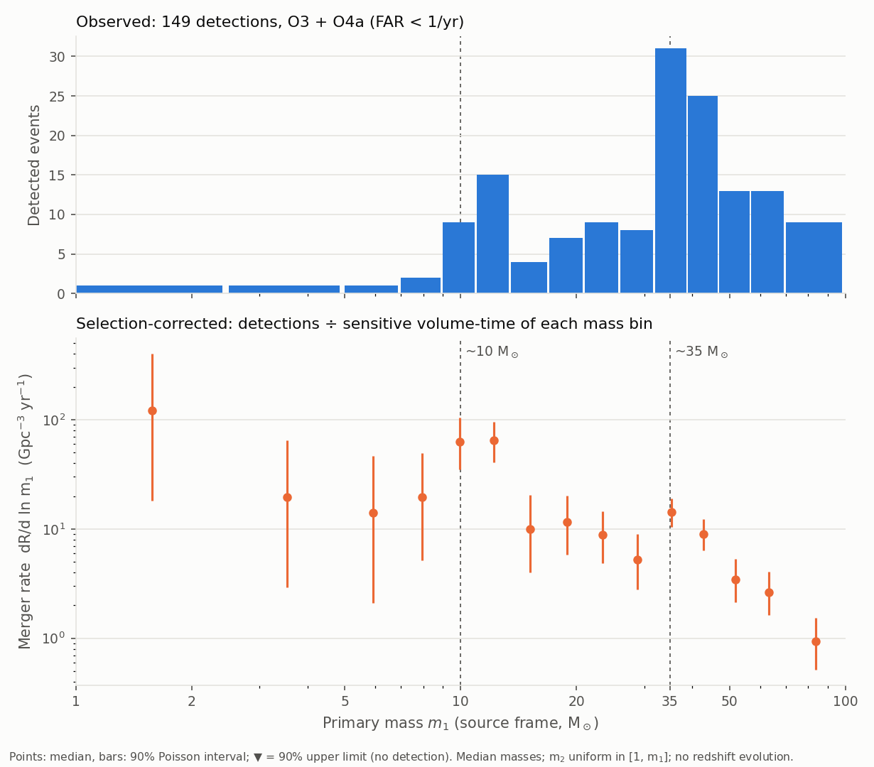
O3 + O4a, 149 candidates with FAR below 1 per year, GWTC-4.0 injections; secondary mass uniform in [1 M☉, m₁], no redshift evolution.

The observed distribution (top) is dominated by BBHs of 30–40 M☉, which are seen to large distances. Once divided by the sensitive volume-time of each bin (bottom), the picture changes: the rate falls by almost two orders of magnitude between 10 and 80 M☉, the peak near 10 M☉ is the strongest feature and the one near 35 M☉ becomes a modest bump. Below 10 M☉ each bin holds one or two events, so the rates there are poorly constrained.

Limitations

• Fixed population shapes: the intervals do not include the uncertainty of the mass, spin and redshift distributions.
• Classification by median masses: events near the 2.5 M☉ boundary (GW230529, with a 2.5–4.5 M☉ primary) may belong to either class.
• All candidates below the FAR threshold are counted as astrophysical; the LVK analyses weight them by their probability of astrophysical origin.