scalar_cloud

Is a binary black hole better fitted with a cloud of an ultralight scalar field around it? The mode refits the public strain of an event with the IMRPhenomXPHM_Scalar waveform of Roy, Vicente, Aurrekoetxea, Clough and Ferreira [100], against the vacuum IMRPhenomXPHM of the catalog, and calibrates the improvement on off-source noise. It reproduces their analysis of GW190728_064510, the event for which they report tentative evidence for a scalar environment.

gwtc_analysis scalar_cloud                                     # GW190728: prepare, first best fit, report (laptop, ~2 h)
# the headline result (\(\mathcal{D}\) = 8.98) needs the samplings, then the fits seeded from them:
gwtc_analysis scalar_cloud --stages sample --executor slurm --submit \
    --python /path/to/env/bin/python --slurm-option=--partition=<partition>
gwtc_analysis scalar_cloud --stages seeded --executor slurm --submit ...   # once the superradiance sampling is done
gwtc_analysis scalar_cloud --stages report                     # once the jobs are done

What comes from the paper, what is added here

The paper's claim is a Bayes factor: nested sampling of the event with the vacuum and the cloud models, under an agnostic and a superradiance prior. It reports no best fit, no background and no p-value. The mode reproduces that analysis and adds a frequentist check around it.

Reproduced from the paper (same model, priors and settings, compared in GW190728_064510):

Element	Source in the paper
the IMRPhenomXPHM_Scalar waveform: torque, dephasing, end of the correction at \(M f_c = 0.018\)	Eq. 2; Supplemental Material (SM) Eq. 6
the agnostic prior: α ≤ (1+q)/2, cloud mass below 0.1 M, uniform density	section on the GWTC-3 events
the superradiance prior for a delay \(\tau_d\)	SM Eqs. 9–10
the binary priors of GWTC-2.1, nested sampling with dynesty in bilby (1000 live points, naccept 60, dlogz 0.1)	analysis settings of the paper, as recorded in scalar_cloud.py
the Bayes factors, the density and α posteriors	ln B ≈ 3.5 (superradiance) and 0.4 (agnostic); Fig. 3 (GW190728), SM Fig. 5 (all events)
the median likelihood gain over the posterior and the chirp-mass posteriors	SM, Fig. 8 and its inset

Done only in gwtc_analysis, and why:

Element	Why
best fits of both models and the deviance \(\mathcal{D}\) = 2 Δln L, the likelihood-ratio test statistic (below)	a Bayes factor costs about a day on 64 CPUs per run; a best fit costs about an hour, so \(\mathcal{D}\) can be computed on the event and on 150 noise segments
fits started from the samples of the superradiance sampling (seeded)	the cloud mode is separate from the vacuum one: fits started from the vacuum best fit miss it (\(\mathcal{D}\) = 0.96 instead of 8.98)
the background: the vacuum best fit injected into 150 off-source segments, p-value	the Bayes factor says which model the data prefer given the priors; it does not say how often noise alone produces such a preference. The background measures that, independently of the prior on the cloud
the sensitivity (an injection–recovery test): the cloud best fit injected into the same segments	tells whether the event's \(\mathcal{D}\) is what a real cloud of that kind would give (it is lower: 4.7% of injections at or below it)
the gain by detector and frequency band	a cloud dephases the whole low-frequency inspiral; a gain concentrated in a narrow band of one detector points to noise rather than to the effect
the agnostic Bayes factor against the upper end of the density prior	the paper does not give that upper end, and the agnostic Bayes factor depends on it
the boson mass in continuous waves	connects the result to the continuous_waves mode

Implementation choices of gwtc_analysis, where the paper does otherwise or does not say:

• the correction is applied to each mode in the J frame, not in the co-precessing frame (identical for aligned spins);
• \(1/(1+\delta)\) is kept, not linearised;
• the agnostic upper end of the density is \(10^9\) g/cm³ (not given in the paper);
• the likelihood has no calibration model and uses the PSDs of the PE file;
• the two cloud samplings of GW190728 used 500 live points instead of 1000 (cost).

These are the likely causes of the remaining differences (a superradiance Bayes factor of 1.3 against 3.5, a density 2 to 4 times lower, a chirp-mass shift of 2.5% against 4.4%): see Against the paper.

The model

An ultralight boson of mass \(m_\phi\) around a binary of total mass \(M\) forms a bound structure of radius \(r_\phi = GM/(c^2\alpha^2)\) (\(M/\alpha^2\) with \(G = c = 1\)), with \(\alpha = G M m_\phi / (\hbar c)\) (the black-hole size over the boson's wavelength; \(\alpha = 0.1\) is \(m_\phi \approx 6.5 \times 10^{-13}\) eV for \(M = 20\,M_\odot\)). In the late inspiral the orbit is well inside it (\(\beta = R / r_\phi \ll 1\)) and the binary ionizes it: it loses angular momentum to the field at the rate (the paper's Eq. 2 and Eq. 6 of its Supplemental Material, \(G = c = 1\))

\[ \dot L_\phi = 4\pi \bar\rho_\phi M^3 \frac{I(v, \alpha, q)}{v^4}, \qquad I = \sum_{\ell, m > 0} \pi^2 \beta^{\frac14 + \frac{\ell}{2}} \left[\frac{2(1+q_2)}{m}\right]^{\frac12 - \ell} \left[1 + (-1)^\ell q_2^{\ell - 1}\right]^2 \left[\frac{Y_{\ell m}(\pi/2, 0)}{\Gamma(\ell + 3/2)}\right]^2 , \]

with \(\bar\rho_\phi\) "the average mass density of scalars in the region \(r \lesssim r_\phi\)" (the paper, after its Eq. 2; the code takes the cloud mass as \(\bar\rho_\phi r_\phi^3\), without a \(4\pi/3\)), \(v = (M\Omega)^{1/3}\), \(\beta = \alpha^2/v^2\), \(q_2 = m_2/M\), and the sum up to \(\ell = 4\) (the \(\ell = 2\) term dominates). Against the gravitational-wave loss \(\dot L_\text{GW} = \frac{32}{5}\eta^2 M v^7\) the orbit shrinks faster by the factor \(1 + \delta\), \(\delta = \frac{5\pi}{8}\,\bar\rho_\phi M^2 I/(\eta^2 v^{11})\), which grows as about \(v^{-13.5}\): the effect sits at the lowest frequencies. In the stationary-phase approximation the phase of the (2, 2) mode changes by

\[ \Delta\Psi_{22}(f) = 2\pi \int_f^{f_c} (f' - f)\, \Delta\!\left(\frac{dt}{df}\right)\!(f')\, df', \qquad \Delta\!\left(\frac{dt}{df}\right) = \left(\frac{dt}{df}\right)_\text{GW}\left[\frac{1}{1+\delta} - 1\right], \]

zero, with its derivative, at the end of the inspiral \(f_c\) (\(M f_c = 0.018\)): only the inspiral changes. Each \((\ell, m)\) mode gets \(\frac{|m|}{2}\Delta\Psi_{22}(2f/|m|)\).

Choice	Here	Note
vacuum model	IMRPhenomXPHM of bilby, as the catalog	\(\bar\rho_\phi = 0\) reproduces it exactly (tested)
where the correction is applied	each mode of SimInspiralChooseFDModes (J frame, seen at θ_JN), rotated into the polarization frame of SimInspiralChooseFDWaveform by a fitted angle	the paper uses the co-precessing frame: identical for aligned spins, an approximation for precessing ones
\(1/(1+\delta)\)	kept, not linearised	identical while \(\delta \ll 1\); finite when the torque exceeds the GW loss
masses in \(\delta\)	source frame (\(\bar\rho_\phi\) is a physical density), redshift from the distance (Planck15)	the kinematics use the detector-frame masses

The dephasing scales roughly as \(\bar\rho_\phi\, \alpha^{2.5}\), i.e. as \(\bar\rho_\phi\, m_\phi^{2.5}\) whatever the mass of the binary. For GW190728 (\(M \approx 20\,M_\odot\)), \(\bar\rho_\phi = 10^6\) g/cm³ and \(\alpha = 0.1\) dephase the (2, 2) mode by about 1.6 rad at 20 Hz and 0.13 rad at 30 Hz.

The test

Best fit. The vacuum model is fitted from the catalog's best samples (Nelder–Mead, the downhill-simplex optimizer, in coordinates whitened by the covariance of the 2000 highest-likelihood samples: the likelihood is too narrow for a plain optimizer). The cloud model has a separate mode, which fits started from the vacuum best fit do not reach: they stay within a few tenths of ln L of vacuum. (In the paper, the cloud posterior sits at a lower chirp mass than the vacuum one, its Fig. 8: a lower chirp mass slows the inspiral, the cloud speeds it up.) The cloud fits therefore start from the 4 best samples of the nested sampling of the event with the superradiance prior (the merger time of each set by a scan of the fixed-time likelihood, the sampling marginalizes it), and are run twice with the binary and the cloud free. The statistic is the deviance \(\mathcal{D}\), the likelihood-ratio test statistic of Neyman and Pearson (called TS in gamma-ray astronomy; \(\Lambda\) in earlier versions of this mode, a name kept as the key Lambda of its result files):

\[ \mathcal{D} = 2\,(\ln \hat L_\text{cloud} - \ln \hat L_\text{vacuum}) \;\ge\; 0 , \]

with \(\ln \hat L\) the log-likelihood ratio of bilby (signal against pure noise) at each model's best fit, at fixed merger time; the noise term cancels in the difference. The cloud model contains vacuum (it is nested), so \(\mathcal{D}\) is positive even without a cloud. For nested models, Wilks' theorem would make \(\mathcal{D}\) follow a χ² distribution with two degrees of freedom (the two extra parameters, \(\bar\rho_\phi\) and α) in noise around a vacuum signal. Two of its conditions fail here: the vacuum value \(\bar\rho_\phi = 0\) is on the boundary of the parameter space (Chernoff 1954), and α is not identifiable when \(\bar\rho_\phi = 0\) (Davies 1977; in particle physics, the look-elsewhere effect). So the distribution of \(\mathcal{D}\) is not assumed: it is measured on noise, below. A first version stopped at a profile of the cloud on a grid of α and of the dephasing at 20 Hz from the vacuum best fit (the profile step, which the fit stage still runs before its polish step): \(\mathcal{D}\) = 0.96 for GW190728, the cloud mode missed.

Background. The vacuum best fit is injected into off-source GWOSC noise, within an hour of the event, and the same procedure is run on each segment: in the background stage from the injected vacuum parameters, in the seeded stage from the same starting points as the event, moved to the time of the injection. The p-value is \((k+1)/(n+1)\) for \(k\) of the \(n\) segments with \(\mathcal{D}\) at least the event's: an empirical (Monte Carlo) p-value, the event counted as one of the trials (e.g. Davison & Hinkley 1997), as the off-source background of GW searches gives their false-alarm rates. The starting points come from the event's own posterior: the background measures how often noise produces, in that region of the parameter space, an improvement as large as the event's, not how often it does so anywhere (the event's sampling searched the whole prior). The p-value is in that sense optimistic.

Bayes factor. The Bayes factor is the ratio of the evidences of the two models, \(B = Z_\text{cloud} / Z_\text{vacuum}\), with \(Z = \int L(\theta)\,\pi(\theta)\,d\theta\) the likelihood averaged over the prior π. ln B > 0 favours the cloud; on the usual scale (Kass & Raftery 1995), ln B of 1–3 is positive evidence, 3–5 strong. Unlike \(\mathcal{D}\), the evidence penalizes the prior volume the extra parameters open (the Occam factor): roughly \(\ln B \approx \Lambda/2 + \ln(\text{posterior volume} / \text{prior volume})\) (Laplace approximation), so it depends on the prior on the cloud. The evidences come from nested sampling (Skilling 2006) with dynesty in bilby: nlive live points explore the prior, naccept 60 accepted steps of the acceptance-walk move replace each one, and the run stops when the remaining evidence is below dlogz 0.1 in ln Z. The cloud model is sampled with two priors on the field. The superradiance prior keeps only clouds that a spinning black hole can grow by superradiance (it amplifies the field's bound waves while the horizon rotates faster than them, losing spin) before the merger, and that have not yet decayed by annihilation into gravitons:

Prior	α	\(\bar\rho_\phi\)
agnostic	uniform, \(0.008 \le \alpha \le (1+q)/2\)	uniform up to \(10^9\) g/cm³ (the paper does not give its upper end), cloud mass \(\bar\rho_\phi r_\phi^3 < 0.1\,M\)
superradiance, delay \(\tau_d\)	\(0.02\,x^{1/9} \le \alpha/(1+q) \le 0.11\,x^{1/15}\), \(x = \frac{m_1}{10 M_\odot}\frac{1\,\text{Myr}}{\tau_d}\): the cloud grew before the merger and did not decay	below the saturation mass, \(1.3 \times 10^8\,\text{g/cm}^3\, \frac{(1+q)^3}{8} \left[\frac{\alpha/(1+q)}{0.07}\right]^7 \left[\frac{10 M_\odot}{m_1}\right]^2\)

The binary priors are those of the GWTC-2.1 analysis. The merger time is marginalized; the distance is sampled (the correction depends on the redshift, so the waveform is not simply proportional to \(1/d_L\)).

Method

The mode runs its own inference on the GWOSC strain of the event: best fits with scipy's Nelder–Mead and nested sampling with bilby's dynesty, on the likelihood of bilby, with the waveform of The model. From the catalog it takes only the settings, the noise spectra and the starting points of the fits; it does not rerun the catalog's parameter estimation. The statistic and the priors are those of The test; here, what each stage computes.

The inputs

• PE file: the event's file of the GWTC PE release on Zenodo (latest version, kept in the PE cache), or --pe-file. From the analysis --pe-label the mode reads the segment length and start, f_low, f_ref, the detectors and their noise spectra (PSDs), the maximum ln L ratio the file records, and the 2000 samples of highest likelihood.
• GWOSC strain: fetched with gwpy at 4096 Hz, resampled to --sampling-frequency and cut to the PE segment. The --n-background off-source segments have the same length, alternately before and after the event, at least 64 s from it and within an hour, inside the GWOSC data of every detector (fewer if the data have gaps).

What the mode does

1. prepare writes these inputs into the work directory, once.
2. Likelihood: bilby's GravitationalWaveTransient with the PE file's PSDs, from f_low to half the sampling frequency, with no calibration model and the PSDs not re-estimated. The fits use the ln L ratio at fixed merger time and vary 13 binary parameters (chirp mass, mass ratio, the six spin parameters, θ_JN, distance, phase, ψ, merger time); the sky position stays that of the starting point.
3. fit (vacuum, profile, polish): the vacuum fit from the best catalog sample, and from the best one in the other mode of the mass ratio if there is one (up to 2500 likelihood calls); the profile on 7 values of α (0.02 to 0.3) × 4 dephasings at f_low (0.5, 2, 8, 30 rad), the density set by bisection, the binary refitted from the vacuum best fit and from starts with the chirp mass lowered by 2, 4 and 6% and the tilts at π/2; then free fits from the 2 best profile points (\(10^2 \le \bar\rho_\phi \le 10^{11}\) g/cm³, \(0.005 \le \alpha \le (1+q)/2\)). A cloud fit below vacuum is replaced by vacuum (\(\mathcal{D}\) = 0).
4. background: in each off-source segment, the vacuum best fit (\(\bar\rho_\phi = 0\)) is injected at the time of the segment and step 3 is rerun, started from the injected parameters.
5. sample: one dynesty run per model of --sample-models (1000 live points, naccept 60, acceptance-walk, dlogz 0.1), the merger time marginalized (prior ±0.1 s around the best catalog sample). The chirp-mass prior is GW190728's, 7.84–12.81 M☉ (detector frame), widened from the PE samples for another event; the distance prior \(\propto d_L^2\) up to 2000 Mpc (twice the largest sample if one is beyond 1500 Mpc). The runs checkpoint every 30 min and resume. ln B is the difference of the ln Z of bilby.
6. seeded: the 25 highest-likelihood samples of the superradiance run, their merger time set by a scan of the fixed-time likelihood (±20 ms in 0.25 ms steps, then ±0.3 ms in 10 µs steps), the 4 best kept as seeds; on the event and on each injection, the vacuum fit, then two Nelder–Mead passes (initial steps 0.1 and 0.05, 2000 calls each) from each seed moved to the time of the injection. The injections of the cloud best fit are not a stage: python -m gwtc_analysis.scalar_cloud seeded --inject cloud.
7. report: the seeded results if present, else those of fit and background. The p-value is \((k+1)/(n+1)\), with \(k\) of the \(n\) background segments at \(\mathcal{D}\) at least the event's.

With --executor slurm (Running on a cluster) the same steps are sbatch chains running scalar_cloud.py itself: slurm/ (vacuum, an array of 28 profile points, polish, an array of background segments; 1 CPU and 3 GB each), slurm_sample/ (one task per model, --npool CPUs, 4 days at most), slurm_seeded/ (the seeds, then an array over the event and the injections). Locally, --jobs runs the profile points, segments and seeded tasks in parallel and sets the sampler pool.

GW190728_064510

On a Slurm cluster (--executor slurm): the vacuum sampling with 1000 live points, the two cloud samplings with 500 (run by hand with python -m gwtc_analysis.scalar_cloud sample --nlive 500; the mode's own samplings use the paper's 1000) (64 CPUs with --npool 64; the default is 32, about a day each), 151 jobs of about an hour for the event and the background, 150 for the injections of the cloud best fit (scalar_cloud.py seeded --inject cloud).

	ln L ratio	Note
catalog maximum-likelihood sample	89.60	96.8 in the PE file (see Limits)
vacuum best fit	91.81	Mc = 10.07 M☉, q = 0.55 (detector frame)
cloud best fit	96.30	Mc = 10.11 M☉, q = 0.58, \(\bar\rho_\phi\) = 5.8 × 10⁶ g/cm³, α = 0.19 (\(m_\phi\) = 1.1 × 10⁻¹² eV), cloud mass 10⁻⁴ M, 38 rad of dephasing at 20 Hz

Result	Here	Roy et al.
deviance \(\mathcal{D}\)	8.98	not used
ln L cloud − ln L vacuum, best fits	4.49 (\(\mathcal{D}/2\))	not given
ln L cloud − ln L vacuum, posterior medians (time-marginalized ln L of the samplings, lower than the fixed-time best fits above)	4.20 superradiance, 4.05 agnostic	≈ 3.7 (Supplemental Material, Fig. 8 inset)
chirp mass (detector frame), posterior median and 90%	vacuum 10.14 (10.05–10.24), superradiance 9.89 (9.73–10.18), agnostic 9.88 (9.72–10.12) M☉	vacuum 10.14 (+0.10/−0.09), cloud 9.69 (+0.27/−0.28) M☉ (Fig. 8)
background	2 of 151 at \(\mathcal{D}\) ≥ 8.98 (the event and one segment with a loud transient, \(\mathcal{D}\) = 112), p = 0.013; 0.007 without that segment; 147 of 150 below 4.1	none (the paper's statistic is the Bayes factor)
injections of the cloud best fit (sensitivity)	\(\mathcal{D}\) = 25 (5–95%: 9.9–44); 4.7% at or below the event's 8.98	none
ln B, superradiance prior (τ_d = 10⁶ yr); ± the statistical uncertainty of the nested-sampling evidences	1.34 ± 0.30	3.5
ln B, agnostic prior (\(\bar\rho_\phi \le 10^9\) g/cm³)	−0.82 ± 0.31	0.4 (upper end of the prior not given)
\(\bar\rho_\phi\), agnostic (90%)	3.2 (0.9–5.9) × 10⁷ g/cm³	≈ 0.7 × 10⁸ (read off Fig. 3, not stated in the text)
\(\bar\rho_\phi\), superradiance	(0.18 ± 0.08) × 10⁸ g/cm³

The agnostic Bayes factor depends on the upper end of the uniform prior on \(\bar\rho_\phi\), which the paper does not give. The posterior lies below \(6 \times 10^7\) g/cm³; lowering the upper end (the prior fraction drawn from the prior itself, the cloud-mass cap barely acts there):

upper end of \(\bar\rho_\phi\) (g/cm³)	10⁹	5 × 10⁸	3 × 10⁸	2 × 10⁸	10⁸	5 × 10⁷
ln B, agnostic	−0.82	−0.16	0.34	0.73	1.40	1.90

The paper's 0.4 corresponds to an upper end near \(3 \times 10^8\) g/cm³.

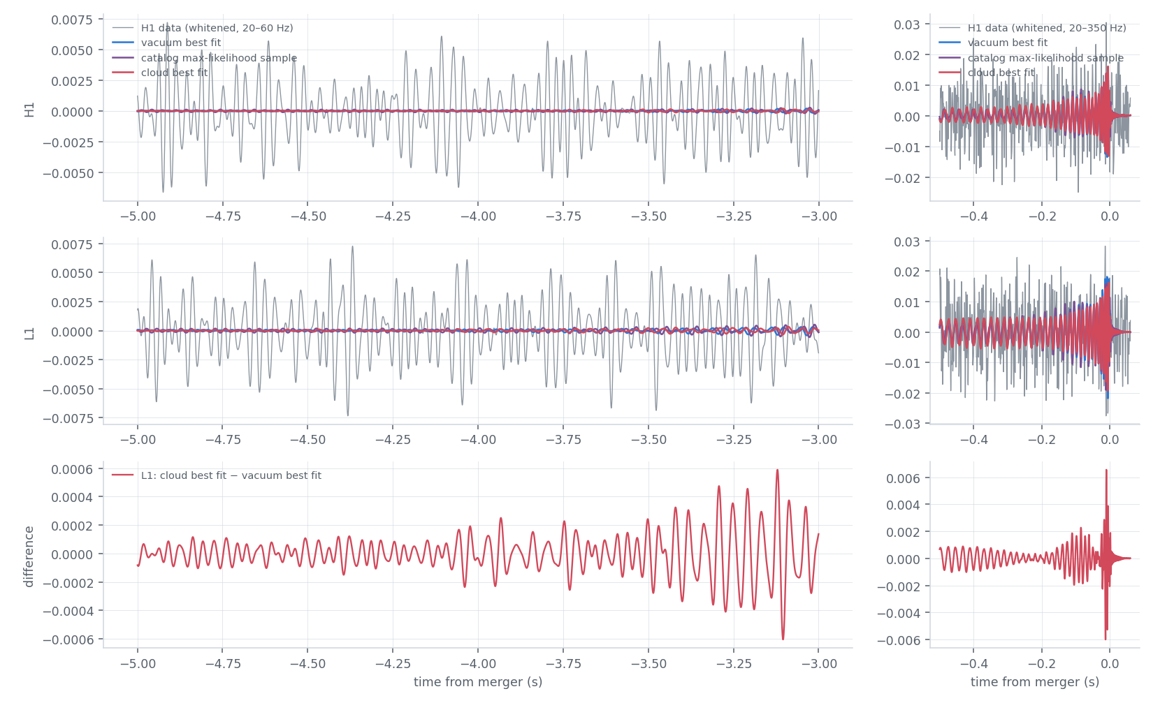
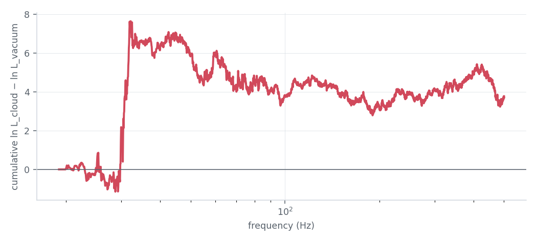
Where the improvement comes from. ln L cloud − ln L vacuum by detector and band:

	20–30 Hz	30–35 Hz	35–60 Hz	> 60 Hz	total
H1	+2.15	+0.31	−0.59	−0.91	+0.96
L1	−0.55	+4.69	−0.40	−0.77	+2.96
V1	−0.15	+0.17	+0.42	+0.12	+0.57
all	+1.45	+5.17	−0.57	−1.56	+4.49

The gain does not accumulate over the inspiral, as a dephasing growing towards low frequencies would: it sits in a few bins between 29.8 and 31.9 Hz, mostly in L1, and the cloud fit is slightly worse than vacuum above 35 Hz. The noise spectra have no line there. A concentration at low frequency is what this cloud would give: with 38 rad of dephasing at 20 Hz, the cloud and vacuum fits are nearly orthogonal below 35 Hz, where the signal has only about 10 of its ≈ 200 units of SNR², and that is where they differ most. Half their squared distance, \(\frac12\lVert h_\text{cloud} - h_\text{vacuum}\rVert^2\), the gain expected from noise-free data holding the cloud signal, is per band:

	20–30 Hz	30–35 Hz	35–60 Hz	> 60 Hz	total
H1	0.89	1.33	0.50	1.69	4.42
L1	3.95	4.03	1.07	1.74	10.79
V1	0.06	0.08	0.62	2.02	2.77

The observed gain follows it in L1 between 30 and 35 Hz only, not below 30 Hz nor in H1. Whether the data around 30 Hz hold a noise fluctuation or the signal is the open question; the background says that noise rarely gives as much near this mode.

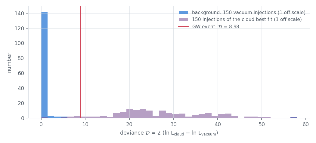
Between two distributions. The same procedure on the event's cloud best fit injected into the 150 off-source segments gives \(\mathcal{D}\) around 25, the density and α recovered without bias (median 8.4 × 10⁶ g/cm³ and 0.16 for 5.8 × 10⁶ and 0.19 injected): 4.7% of these injections give \(\mathcal{D}\) ≤ 8.98. The event is above what noise gives around vacuum (p ≈ 0.01) and below what this cloud would give (≈ 5%): a weaker effect, or a noise fluctuation at 30 Hz on a vacuum signal, fits both better than the best-fit cloud.

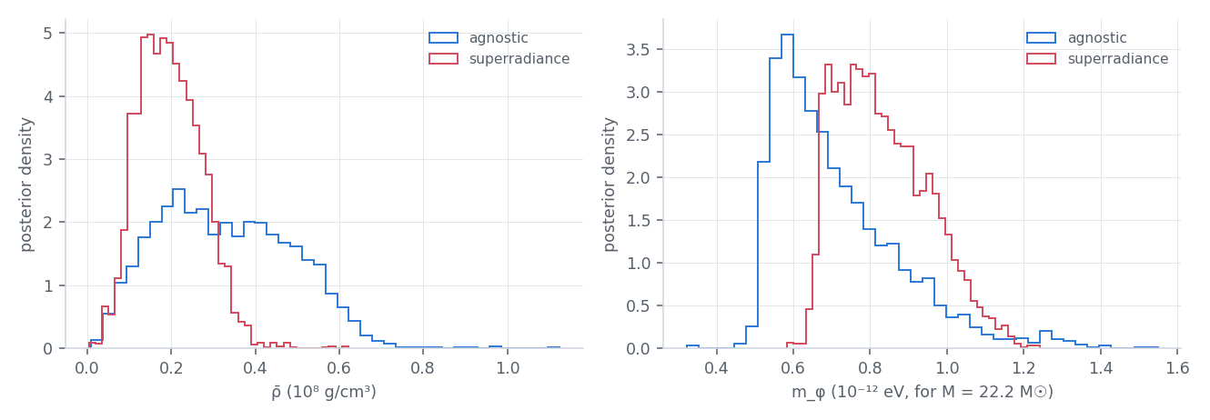
Against the paper. The paper's statistic is the Bayes factor: it gives no best fit, no background and no p-value, so \(\mathcal{D}\), the background and the injections have no published counterpart. What can be compared: a cloud mode with a density of 10⁷ g/cm³ and α of a few 0.1; a median likelihood gain over the posterior of 4.2 (superradiance) and 4.05 (agnostic), against the paper's 3.7 (the best-fit gain, 4.49, is a maximum, not comparable); an agnostic Bayes factor that matches theirs for a prior up to about \(3 \times 10^8\) g/cm³; but a smaller Bayes factor with the superradiance prior (1.3 against 3.5) and a density 2 to 4 times lower. The chirp-mass shift is reproduced in the posteriors, smaller: the vacuum posterior, 10.14 M☉ (detector frame), is the paper's exactly (which places its values in the detector frame too), and the cloud posteriors sit at 9.89 M☉, 2.5% below it, against 4.4% below (9.69 M☉) in the paper. The cloud best fit (10.11 M☉) is not in the bulk of the cloud posterior: the fits find the highest point of the cloud mode, the posterior weighs its volume. Differences that can contribute: the frame of the correction (J frame here, co-precessing there), the PSDs and the likelihood (ln L 7 below the PE file's), 500 live points instead of 1000, and the normalisation of the torque, which sets the density for a given dephasing.

The same boson in continuous waves

Per sample (each with its own source-frame mass), the scalar mass is \(m_\phi = 0.89\) (90%: 0.70–1.17) × 10⁻¹² eV with the superradiance prior and 0.73 (0.56–1.14) × 10⁻¹² eV with the agnostic one. A cloud of such bosons around an isolated spinning black hole would annihilate into a continuous wave at \(2 m_\phi c^2/h\) = 340–570 Hz, inside the band of the LVK all-sky search for boson clouds in O3 (20–610 Hz). That search excludes, at these masses, young clouds around light black holes (8–28 M☉) out to some kpc, but says nothing of a cloud carried by a binary, and its limits constrain the boson only together with a model of the Galactic black holes. The continuous_waves mode draws its exclusions with this band.

The same boson and black-hole spins

Superradiance spins black holes down, so fast-spinning black holes in the right mass range exclude the boson. The paper discusses this in its Discussion [100]:

• the high spins of black holes in X-ray binaries "have been interpreted as excluding scalars in this mass range", but "these spin estimates, however, are highly model-dependent": a warm Comptonization layer in Cygnus X-1 "can reduce the inferred spin parameter to a/M ≲ 0.1" (Zdziarski et al. 2024, ApJL 967, L9);
• the spins of a few black holes measured through gravitational waves "do not exclude the full range favored by our analysis of GW190728; the main tension arises from GW190517, whose spin measurement disfavors \(m_\phi \lesssim 1.1 \times 10^{-12}\) eV";
• "joint spin measurements from the full GWTC-2 showed weak evidence for a light scalar in the mass range suggested by our analysis" (Ng et al. 2021).

The band found here, 0.70–1.17 × 10⁻¹² eV, lies mostly below that value: only its upper end escapes the GW190517 constraint. The tension concerns the boson, not the fit, and the mode does not test it.

Limits

• The torque is Newtonian and valid for \(\beta \ll 1\); close to the merger the model is extrapolated, and the correction is switched off there.
• A large \(\mathcal{D}\) means that the vacuum model fits the inspiral worse than usual. Eccentricity, waveform systematics, calibration or a noise feature at low frequency can do the same: \(\mathcal{D}\) is a ranking statistic, as in a search, and its p-value says only that vacuum fits unusually badly; the Bayes factor under a physical prior is the actual claim.
• This likelihood gives ln L = 89.6 at the catalog's best sample of GW190728, against 96.8 in the PE file: the phases agree in every detector, the difference comes from the noise-spectrum, window and calibration handling. Both models use the same likelihood, so the comparison is not affected.

Outputs

• The HTML report ends with the PE files of this run (recorded in event.json by prepare): for each event the file read, its type (nocosmo, cosmo, combined or the GW170817 bundle) and where it was taken from (Zenodo, the S3 mirror, Galaxy, a PE cache), then the options of the run; see Which PE file is read;
• --out-report (HTML): the fits, the background and the posteriors, with the plots;
• --out-summary (TSV): the fits (vacuum and cloud), with \(\mathcal{D}\) and its p-value;
• <workdir>/: event.json (the event and its priors), the results of each stage, and plots/ (whitened.png, lnl_by_frequency.png, dephasing.png, profile.png, background.png, cloud_posteriors.png).

Options

Option	Default	Meaning
--event	GW190728_064510	the event (name of the GWTC PE releases)
--pe-file, --pe-label	the event's Zenodo file, C01:IMRPhenomXPHM	settings, noise spectra and starting points
--workdir	scalar_cloud	work directory
--stages	prepare fit report	among prepare fit background sample seeded report (seeded: the event and the background with the cloud fits started from the superradiance sampling, which it needs)
--sampling-frequency	2048	Hz
--n-background	150	off-source injections
--jobs	1	local parallel processes (fit, background, seeded), sampler pool (sample)
--sample-models	vacuum agnostic superradiance	models of the sample stage
--tau-d	10⁶	superradiance prior: years between black-hole formation and merger
--executor	local	slurm: the heavy stages as sbatch scripts in <workdir>/slurm, <workdir>/slurm_sample and <workdir>/slurm_seeded
--python, --slurm-option, --slurm-env-setup, --submit	this interpreter; none; none; off	Slurm: the jobs' interpreter, extra #SBATCH options, setup lines, submission
--npool	32	Slurm: CPUs of each sampling job
--out-report, --out-summary	scalar_cloud.html, scalar_cloud.tsv	report and table of the fits
--data-repo {zenodo,s3,galaxy}	zenodo	where the PE file are downloaded from: their public sources, or a mirror holding the same files, s3 (the MinIO bucket, faster) or galaxy (the public usegalaxy.org history), else the public source (S3 mirror of the public files)

Cost for GW190728 (16 s at 2048 Hz): a vacuum likelihood 0.035 s, a cloud likelihood 0.2 s (the modes of LAL). The best fit takes about 2 CPU-hours, each background injection about 2 (1 with seeded), the nested sampling of the cloud models about a day on 64 CPUs with 500 live points (a cluster job).