Waveform models

Every number derived from a GW event, the masses, spins, distance, sky map and everything built on them, comes from comparing the data with waveform models: for a given source (masses, spins, orientation, distance, and possibly tides, eccentricity or an environment) a model returns the two polarizations h₊(t) and h×(t) the detectors should record. Parameter estimation evaluates millions of them, so the posterior samples of every catalog event are conditional on a waveform model. General relativity fixes the signal of two black holes completely, but there is no closed formula for it: the models are approximations, each including some physics and not other. This page explains what the models contain, how their names encode it, how they evolved from GW150914 to GWTC-5.0, and which ones gwtc_analysis reads.

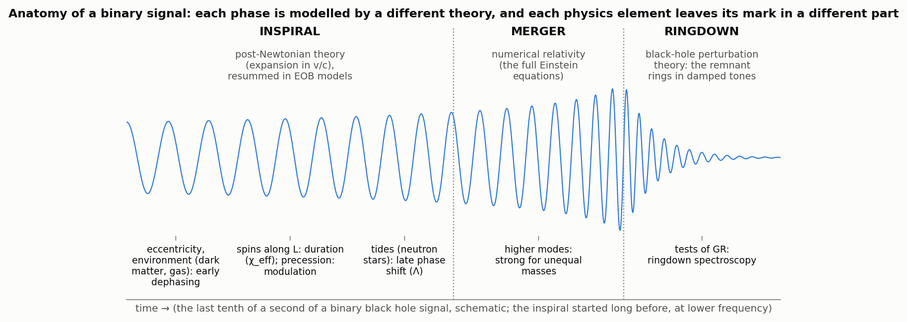
The three phases of a binary signal and the theory that describes each: post-Newtonian expansions for the inspiral, numerical relativity for the merger, black-hole perturbation theory for the ringdown; below, where each physics element leaves its mark (schematic).

Three ways to build a model

All three answer the same question, the signal of two compact objects in general relativity, but they trade accuracy, speed and coverage of the parameter space differently. An analogy: numerical relativity is the wind-tunnel measurement, effective-one-body is a physical theory with a few constants tuned to the wind tunnel, and phenomenological models are engineering formulas fitted to the measurements and to that theory.

Numerical relativity (NR): solving Einstein's equations directly. The full equations are evolved on a computational grid, from a few orbits before merger to the settled final black hole. No approximation beyond the numerical resolution: this is the reference, and the only way to get the merger itself right. Possible since 2005 (Pretorius [115]; then the "moving puncture" method, Campanelli et al. [116] and Baker et al. [117]). Main codes: SpEC (the SXS collaboration, whose public catalog holds thousands of simulations [118]), the Einstein Toolkit, BAM, GRChombo. The price: weeks to months of supercomputer time per simulation, for the last tens of orbits only, at one point of parameter space. Long inspirals (a binary neutron star spends thousands of cycles in the band), very unequal masses and extreme spins are expensive or out of reach. NR is therefore never run inside parameter estimation: it is the ground truth the other families are built from and checked against.

NR surrogates (NRSur): interpolating the simulations. A surrogate decomposes a set of simulations on a compact basis and fits how the coefficients vary with mass ratio and spins, so it returns a new waveform between the simulations in a fraction of a second. Within its training range it is as accurate as NR itself (NRSur7dq4 [98]: mass ratio up to 4, spins up to 0.8, precession and higher modes included). Outside it, it has nothing to say, and it is only as long as the simulations (about 20 orbits), which covers the whole signal in the detectors only for heavy binaries, roughly above 60 M☉ in total.

Effective-one-body (EOB: SEOBNR, TEOBResumS): a physical model of the dynamics. Buonanno and Damour [94] map the two-body problem onto one effective body of reduced mass μ = m₁m₂/M moving in a deformed black-hole spacetime, the deformation growing with the symmetric mass ratio ν = μ/M. When one body is much lighter (ν → 0) this is exactly a particle orbiting a black hole; for comparable masses the post-Newtonian results are built into the deformation in a resummed form, which stays well behaved close to merger where the plain post-Newtonian series breaks down. The orbit is then evolved in time: an energy (Hamiltonian) gives the motion, a resummed gravitational-wave flux removes energy, the waveform is computed along the orbit, and at the peak the merger is joined to the ringdown (the quasinormal modes of the final black hole). The few unknown higher-order terms are calibrated to numerical relativity ([95], [96], [97]). Strengths: accurate over the whole inspiral, however long, from equal masses to extreme mass ratios; new physics enters naturally in the dynamics (tides, eccentricity, spin precession). The price: an ordinary differential equation integrated in time, slower than a formula, hence the reduced-order versions (ROM) and the faster SEOBNRv5 implementation [121].

Phenomenological (IMRPhenom): a fitted formula for the signal itself. Started by Ajith et al. [119]. Instead of evolving an orbit, the model writes the amplitude and phase directly, usually as functions of frequency, in pieces: an inspiral part (post-Newtonian plus extra fitted terms), an intermediate part, and a merger–ringdown part shaped around the ringdown frequency of the final black hole. The coefficients are fitted, across mass ratio and spin, to hybrid waveforms: an EOB or post-Newtonian inspiral glued to an NR merger. Precession is added by "twisting up" [120]: an aligned-spin waveform is rotated with time-dependent angles that follow the precessing orbit (the P in the names). Strengths: closed formulas in the frequency domain, where the likelihood is computed, so a waveform costs milliseconds; this is why the catalogs run their large analyses with IMRPhenomXPHM [51]. The price: the accuracy is that of the fit and of the twisting approximation; outside the calibration set (high mass ratio, large tilted spins) the fit is an extrapolation.

How they relate. NR is the reference; EOB is calibrated to NR; Phenom is fitted to EOB + NR hybrids; surrogates interpolate NR (or, as ROM, an EOB model). The differences between models are therefore not independent opinions but a measure of the remaining systematic error. Where it matters, for loud, heavy, precessing or unequal-mass signals, the LVK analyses an event with two families (Phenom and EOB) and combines the samples (the Mixed labels, below). When they disagree, the model, not the noise, limits the measurement: GW231123 is the current example (below).

	Numerical relativity	NR surrogate	Effective-one-body	Phenomenological
Method	Einstein's equations solved on a grid	interpolation of NR simulations	effective-body dynamics evolved in time	fitted closed formulas, mostly in frequency
Accuracy	reference	NR-level inside its range	high, calibrated to NR	good, limited by the fits
Cost of one waveform	weeks–months of supercomputer	~0.01–0.1 s	~0.1–1 s (faster with ROM)	~milliseconds
Length	last tens of orbits	~20 orbits	any	any
Coverage	discrete simulations	inside the training range only	all masses and mass ratios	all, but extrapolates outside the calibration set
Used for	building and testing models; exotic physics	heavy binaries (GW190521, GW231123)	cross-checks, eccentricity, tides, extreme mass ratios	the bulk of catalog parameter estimation

Two related tools are not catalog models: post-Newtonian approximants such as TaylorF2 (inspiral only, used for binary neutron stars and in searches), and numerical relativity itself, described above.

The physics elements

Physics element	What it does to the signal	Marker in the names	Examples
masses	the frequency sweep and duration (chirp mass), the merger frequency	all models	—
spins along the orbital angular momentum L	lengthen or shorten the inspiral (χ_eff), change the merger	aligned-spin models	IMRPhenomD, IMRPhenomXAS, SEOBNRv4
precession (spins tilted against L)	the orbital plane wobbles around the total angular momentum J: amplitude and phase are modulated (χ_p)	P	IMRPhenomPv2, IMRPhenomXP, SEOBNRv4P
higher modes (multipoles beyond the (2,2) quadrupole)	extra harmonics, strong for unequal masses and inclined orbits; they help measure the inclination	HM	IMRPhenomXHM, IMRPhenomXPHM, SEOBNRv4PHM, SEOBNRv5PHM
better precession dynamics	spin evolution integrated from the post-Newtonian equations, or tuned to numerical relativity	SpinTaylor, PNR, XO4a	IMRPhenomXPHM-SpinTaylor [52], IMRPhenomXPNR, IMRPhenomXO4a
tides (neutron stars)	an extra phase shift at the end of the inspiral, set by the tidal deformability Λ	NRTidal, T	IMRPhenomPv2_NRTidal(v2) [66], SEOBNRv4T
tidal disruption (neutron star–black hole)	the neutron star is torn apart and the signal shuts off early	NSBH	IMRPhenomNSBH, SEOBNRv4_ROM_NRTidalv2_NSBH
eccentricity	a burst at each closest approach, extra harmonics, a faster inspiral	E, Dalí	TEOBResumS-Dalí, SEOBNRv5EHM (research models: the catalogs assume circular orbits)
environment (gas, dark matter)	extra dephasing in the inspiral, largest at low frequency	added terms	IMRPhenomXPHM_Scalar, a scalar cloud around GW190728 (Roy et al. [100]; not an LVK model)
deviations from general relativity	shifted post-Newtonian, merger or ringdown coefficients	parametrized versions	parametrized IMRPhenom (TIGER, FTI), pSEOBNR; ringdown-only fits (pyRing)

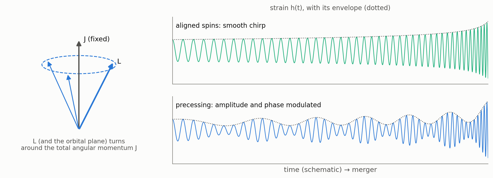
Precession: with tilted spins, the orbital angular momentum L turns around the fixed total angular momentum J, and the signal is modulated (schematic).

Gravitational waves round off orbits (Peters 1964 [99]): a binary radiates most at closest approach, which shrinks the far side of the orbit, so the eccentricity falls as the binary shrinks, roughly as f^(−19/18). Binaries from two stars that evolved together arrive in the band essentially circular; binaries assembled dynamically (dense star clusters, galactic nuclei, AGN disks) can keep a measurable eccentricity, which is why eccentricity, like precession, is a clue to how a binary formed. The two are easily confused in short signals: GW190521 has been read both as eccentric and as strongly precessing.

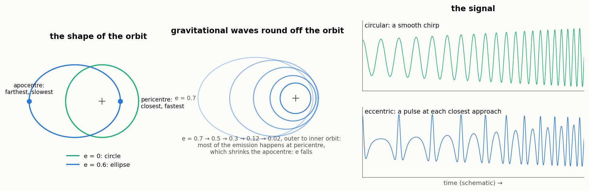
Eccentricity (schematic): a circular and an eccentric orbit; the orbit becoming round as it radiates; a smooth chirp against a pulse at each closest approach.

Decoding the names

The names are compact descriptions: a family, a generation or version, then letters for the physics included.

Taylor approximants (post-Newtonian, inspiral only). The inspiral is computed from energy balance: the orbital energy and the radiated flux are both known as series in the orbital speed v/c, and "Taylor" means they are used as Taylor series in v (as opposed to resummed forms such as the older Padé approximants).

• TaylorT1–T4: time-domain variants, which differ only in how the energy balance is solved or re-expanded.
• TaylorF2: frequency domain, the phase written directly as a function of frequency with the stationary-phase approximation; analytic and fast, used for long binary-neutron-star signals and in searches.
• SpinTaylorT4, T5: the T4 or T5 inspiral plus the post-Newtonian equations that make the spins and the orbit precess. IMRPhenomXPHM-SpinTaylor takes its precession angles from integrating these equations.

IMRPhenom. IMR = Inspiral–Merger–Ringdown, the whole signal; Phenom = phenomenological. The letter is the generation: A, B, C (2007–2010, the first complete models, non-spinning then aligned spins), D (2016, accurate aligned spins), Pv2 and Pv3 (precession, by "twisting" an aligned-spin model with time-dependent angles), the X family (2020–: XAS aligned spins, XHM higher modes, XP precessing, XPHM both), T (the same physics in the time domain, e.g. IMRPhenomTPHM), XO4a (prepared for the O4a run, with precession tuned to numerical relativity), XPNR (precession calibrated to numerical relativity). Suffixes add physics: HM, _NRTidal(v2), NSBH, -SpinTaylor.

SEOBNR. S = Spinning, EOB = Effective-One-Body, NR = calibrated to Numerical Relativity; then the version (v2 to v5), P precessing, HM higher modes, T tides, E eccentric, and _ROM a reduced-order model, a fast frequency-domain surrogate of the EOB model itself.

TEOBResumS. T = Tidal, EOB = Effective-One-Body, Resum = resummed (the post-Newtonian series rewritten in closed forms that behave better near merger), S = Spins. TEOBResumS-Dalí is its version for eccentric and generic orbits.

NRSur. NR = trained on Numerical-Relativity simulations, Sur = surrogate; then the number of source parameters (d) and the largest mass ratio (q): NRSur7dq4 covers 7 parameters (the mass ratio and the six components of the two spins) up to q = 4; NRHybSur3dq8 is a hybrid (numerical relativity joined to a post-Newtonian inspiral) with 3 parameters (mass ratio and two aligned spins) up to q = 8.

Labels in the PE files. A label such as C00:IMRPhenomXPHM-SpinTaylor is one analysis of the event: C00, C01 give the version of the detector calibration it used, then the waveform model. Mixed combines the samples of two or more models equally, which folds their difference into the posterior. HighSpin and LowSpin are the spin priors of neutron-star analyses (spins up to large values, or limited to those of known pulsars in binaries).

How the models evolved, catalog by catalog

Release	Models	The question that drove them
GW150914 (2016)	IMRPhenomPv2, SEOBNRv2 (aligned spins), compared with numerical relativity	is it two black holes, and how heavy?
GW170817 (2017)	TaylorF2, IMRPhenomPv2_NRTidal, low- and high-spin priors	tides: the neutron-star equation of state
GWTC-1 (O1–O2, 2018)	IMRPhenomPv2, SEOBNRv3 (precessing), NRTidal for the neutron stars	spins and precession across a population
GWTC-2 (O3a, 2020)	IMRPhenomPv3HM, SEOBNRv4PHM; NRSur7dq4 for GW190521	higher modes became necessary with unequal-mass events (GW190412, GW190814)
GWTC-2.1, GWTC-3 (O3, 2021)	IMRPhenomXPHM and SEOBNRv4PHM, combined as Mixed; IMRPhenomNSBH and SEOBNRv4_ROM_NRTidalv2_NSBH for the neutron-star–black-hole events	faster, more accurate precessing models for ~90 events
GWTC-4.0 (O4a, 2025)	IMRPhenomXPHM-SpinTaylor and SEOBNRv5PHM for the binary black holes (and Mixed); NRSur7dq4 for 44, IMRPhenomXO4a for 28; IMRPhenomNSBH and IMRPhenomPv2_NRTidalv2 for neutron-star events	louder signals need better precession; the heaviest need surrogates
GWTC-5.0 (O4b, 2026)	IMRPhenomXPHM-SpinTaylor, IMRPhenomXPNR and SEOBNRv5PHM for the binary black holes; NRSur7dq4 for 53	precession tuned to numerical relativity; several models per event to measure the systematics

The O4 rows are counted from the public PE files of the two releases; the earlier ones are the models of the catalog papers.

When the models disagree. For loud or heavy events the difference between models can be as large as the statistical uncertainty. GW231123, the most massive binary of GWTC-4.0, is the clearest case: its multipole and precession signal-to-noise ratios differ by a factor of three to four between models (parameters_estimation), and the cosmology analyses leave it out.

New questions, new models

• Environments and dark matter. A binary in a dense medium loses energy and angular momentum faster than in vacuum, so its phase drifts from the vacuum prediction, mostly early in the inspiral. Roy et al. [100] built IMRPhenomXPHM_Scalar, IMRPhenomXPHM plus a Newtonian dynamical-friction torque from a scalar cloud, and re-analysed the public strain of 28 binary black holes: ln B ≈ 3.5 in favour of the environment for GW190728 alone, a tentative result. The scalar_cloud mode repeats that fit: ln B = 1.34 ± 0.30 with the superradiance prior and −0.82 ± 0.31 with the agnostic one. Such models cannot reuse the catalog posterior samples, which assume the vacuum model: the strain has to be analysed again.
• Eccentricity models (TEOBResumS-Dalí, SEOBNRv5EHM) would test dynamical formation directly.
• Tests of general relativity add free deviations to the coefficients of the models, or fit the ringdown tones alone; the area-theorem test of GW250114 uses NRSur7dq4 (area_law).
• Lensing is not part of the waveform model: magnification, time delay and phase shift are applied to the signal afterwards.

The waveform models in gwtc_analysis

gwtc_analysis reads the posterior samples of the public releases; it re-runs parameter estimation only in scalar_cloud, which fits the strain of one event itself. The waveform behind each result is the label it reads:

Mode	Label read (default)	Choose another
catalog_statistics, event_selection	the GWOSC catalog values (the medians the catalog publishes)	—
parameters_estimation	Mixed for the posteriors; the strain overlay is synthesized with the waveform engine of the label	--pe-label, --waveform-engine; the report compares the multipole and precession SNRs of all the labels
search_skymaps	the Mixed skymap, else IMRPhenomXPHM-SpinTaylor (GWTC-5.0 has no Mixed maps)	--skymap-label
hubble_constant, spin_population	one model per event, as the LVK cosmology analyses: IMRPhenomXPHM-SpinTaylor (O4), IMRPhenomXPHM (O1–O3)	—
hubble_constant --method bright, counterpart, neutron_star_eos	IMRPhenomPv2_NRTidal, low-spin prior (high spin also reported)	--pe-label (bright, counterpart), --spin-prior (neutron_star_eos)
area_law	the LVK release: NRSur7dq4 on data truncated before the peak for the initial areas, ringdown quasinormal-mode fits for the remnant	—
lens_pairs	IMRPhenomXPHM, as hubble_constant	—
scalar_cloud	its own fits of the strain, IMRPhenomXPHM against IMRPhenomXPHM_Scalar, set up from the C01:IMRPhenomXPHM PE analysis	--pe-label

Using a single model per event, rather than a mixture, avoids combining samples drawn with different priors (for instance on the luminosity distance), which the reweighting of the population analyses would otherwise have to handle; it is the choice of the LVK cosmology analyses.