stochastic

The background of unresolved compact binaries, Ω_GW(f), predicted from the catalog and compared with the upper limits of the stochastic searches.

gwtc_analysis rates --out-rates merger_rates.tsv
gwtc_analysis stochastic --spectral-posterior hubble_constant_spectral --rates merger_rates.tsv

Inputs

The calculation combines two earlier results: a merger rate today (from rates) and its evolution with redshift and mass distribution (from a hubble_constant run). Run those two modes first. What each input provides, and the other choices: Options.

# the inputs, from the same release: rates and a Power Law + Peak spectral siren (both GWTC-4.0)
gwtc_analysis rates --sensitivity-release gwtc4 --out-rates rates_gwtc4.tsv
gwtc_analysis hubble_constant --workdir h0_plp --stages prepare sample combine reweight \
    --icarogw-python ~/.conda/envs/icarogw/bin/python --seeds 1 2 3 4
# the background, with the fitted rate shape kept beyond the detected events as a check
gwtc_analysis stochastic --spectral-posterior h0_plp --rates rates_gwtc4.tsv --high-z posterior --n-draws 400

Method

The energy density of the background per logarithmic frequency, in units of the critical density ρ_c c² = 3H₀²c²/(8πG), is (Phinney 2001 [83])

\[ \Omega_\text{GW}(f) = \frac{f}{\rho_c c^2} \int_0^{10} dz\, \frac{R(z)\, \langle dE/df_s \rangle\big(f(1+z)\big)}{(1+z)\, H(z)}, \]

with R(z) the merger rate per comoving volume and source-frame time, and ⟨dE/df_s⟩ the energy spectrum of one merger averaged over the population (Planck15, as the volumes of the rates mode).

Population	Rate	Masses	Spectrum
BBH	R(0.2) of rates (25.2 Gpc⁻³ yr⁻¹ with its default release, gwtc5), times the Madau–Dickinson shape of each spectral-siren draw	the mass model of each draw: Power Law + Peak or Multi Peak	inspiral–merger–ringdown, Ajith et al. 2008 [84]
BNS	R(0) of rates, star-formation history [16]	uniform 1–2.5 M☉	inspiral to the ISCO
NSBH	R(0) of rates, star-formation history	m_BH ∝ m^−2.35 on 2.5–40 M☉, NS uniform 1–2.5 M☉	inspiral to the ISCO

The BBH rate is normalized at z = 0.2, where the catalog measures it best. Beyond the farthest detected events (z_h ≈ 1, from the work directory) the fitted shape is only its prior: by default the rate follows the star-formation history there, joined continuously at z_h (--high-z sfr); --high-z posterior keeps the fitted shape up to z = 10.

What the mode does

The mode runs no inference and reads no strain. It reads two products of earlier runs of the package, the posterior of a hubble_constant spectral siren and the rates TSV of rates, and evaluates the integral above for draws of them.

1. Inputs. The posterior is posterior_reweighted.tsv of the work directory, else posterior.tsv, or the TSV given; the mass model is recognized from its columns. From the rates TSV: the 5%, 50% and 95% values of the BNS and NSBH rates and of the BBH rate at its reference redshift (the BBH row with z_ref > 0).
2. Horizon. \(z_h\) is the redshift (Planck15) of the largest median distance among the events of the run's inputs.h5, else 1; it must exceed the reference redshift of the BBH rate.
3. BBH, per draw. --n-draws rows of the posterior (fixed seed). For each: 1500 binaries drawn from its mass model (\(m_1\) by inverting the cumulative distribution on a grid, \(m_2 \mid m_1 \propto m_2^\beta S(m_2)\)), their mean Ajith et al. spectrum on 600 frequencies from 1 Hz to 30 kHz (zero above); a rate at the reference redshift drawn from a log-normal matching the median and 90% interval of rates, times \(\psi(z)/\psi(z_\text{ref})\) with the draw's γ, κ, z_p. With --high-z sfr the shape beyond \(z_h\) is that of Madau & Dickinson 2014 (γ = 2.7, κ = 2.9, z_p = 1.9), scaled to be continuous at \(z_h\).
4. BNS and NSBH. One mean inspiral spectrum from 20 000 binaries each, the integral for a rate of 1 Gpc⁻³ yr⁻¹ following the star-formation shape, then scaled by log-normal draws of the local rate, independent of the BBH draws.
5. Integral. Trapezoids over 400 redshifts from 0 to 10, at 120 frequencies from 5 to 3000 Hz, with H₀ and \(E(z)\) of Planck15. The total is summed draw by draw; the medians and 90% bands are percentiles of the draws.
6. Other high-z choice. The BBH part at 25 Hz only, with at most 100 draws, quoted in the report.

The upper limits and the LVK prediction are constants of the code (2.0 × 10⁻⁹ at 25 Hz, index 2/3, drawn from 20 to 90.6 Hz; 3.4 × 10⁻⁹ for O3; 6.3 (+5.0 / −2.2) × 10⁻¹⁰), not recomputed from search data. The numbers of mergers of In numbers of mergers are not an output of the mode.

Results

GWTC-4.0 Power Law + Peak posterior, with the rates of the default rates release (gwtc5, O3–O4b: BBH 25.2 at z = 0.2). With the gwtc4 rates of the example above (BBH 26, BNS 43, NSBH 54) the BNS and NSBH parts grow in proportion:

Population	Ω_GW(25 Hz), median (90%)
BBH	6.0 × 10⁻¹⁰ (4.3–9.3 × 10⁻¹⁰)
BNS	0.3 × 10⁻¹⁰ (0.06–1.8 × 10⁻¹⁰)
NSBH	0.9 × 10⁻¹⁰ (0.4–2.2 × 10⁻¹⁰)
total	7.5 × 10⁻¹⁰ (5.5–11.7 × 10⁻¹⁰)
LVK prediction from GWTC-5.0 [85]	6.3 (+5.0 / −2.2) × 10⁻¹⁰
upper limit, data through April 2025 [85]	≤ 2.0 × 10⁻⁹ (95%, index 2/3)
upper limit, O3 [86]	≤ 3.4 × 10⁻⁹

The prediction agrees with the LVK one and lies a factor 2.7 below the current upper limit.

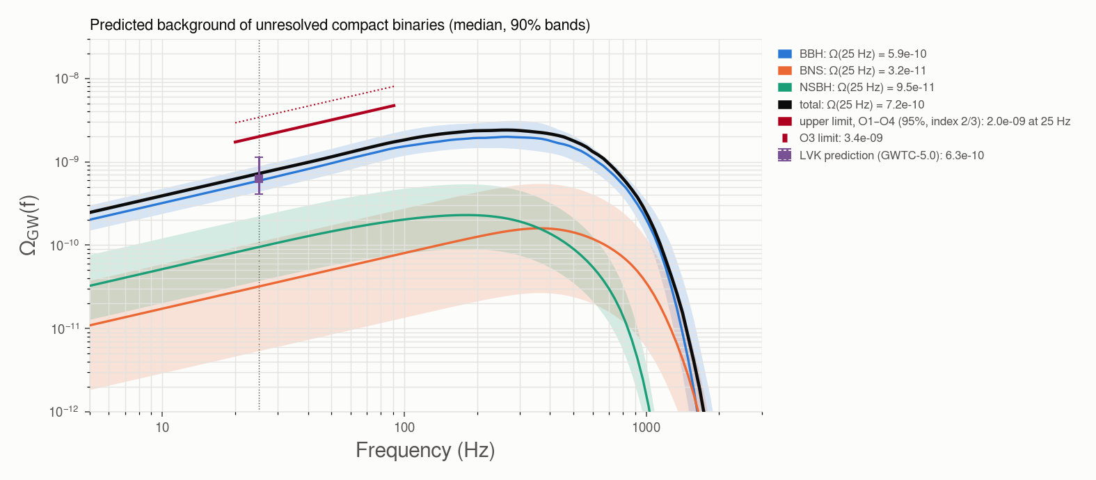
Below ~100 Hz the background grows as f^2/3 (the inspiral), in the band where the searches are most sensitive; the BBH spectrum turns over at the merger frequencies of the redshifted masses.

In numbers of mergers

The same rates, integrated over the whole sky and redshift, \(\dot N = \int R(z)\, \frac{dV_c}{dz}\, \frac{dz}{1+z}\) (the 1 + z is the time dilation: mergers per year of our time), with the rate history of the background: the star-formation history for BNS and NSBH, the fitted Madau–Dickinson shape for BBH up to z_h ≈ 1 and the star-formation history beyond. Rates: BNS 26 [4, 87] and NSBH 33 [13, 67] Gpc⁻³ yr⁻¹ today, BBH 25.2 at z = 0.2 (rates --sensitivity-release gwtc5, median [90%]).

	Local rate (Gpc⁻³ yr⁻¹)	Whole Universe (z < 10), one every	z < 1, one every	Within 40 Mpc, one every	Detected per year	Ω_GW(25 Hz)
BBH	25 at z = 0.2	~6 min (3.5–9)	~70 min	—	~96 (248 in 2.59 yr)	6.0 × 10⁻¹⁰
NSBH	33 [13, 67]	~4 min (2–10)	~40 min	~110 yr (56–290)	~1.5 (4 in 2.59 yr)	0.9 × 10⁻¹⁰
BNS	26 [4, 87]	~5 min (1.5–33)	~50 min	~140 yr (43–930)	~0.4 (1 in 2.59 yr)	0.3 × 10⁻¹⁰

90% ranges from the rate intervals (BNS, NSBH) or from 300 draws of the Madau–Dickinson shape of a Power Law + Peak posterior with R(0.2) fixed (BBH, so its range is too narrow by about ±10%). Detected: the candidates of O3, O4a and O4b used by rates (FAR < 1/yr).

• The three populations merge about as often, one every few minutes each in the observable Universe: about 10⁵ per year each. About 90% of these mergers are beyond z = 1, where the rate is the assumed star-formation history, not a measurement.
• What differs is how far they are seen. A BBH is detected out to a few Gpc, an NSBH to a few hundred Mpc, a BNS to ~160 Mpc (the O4 range): BBHs dominate both the detections and the background. The rest, more than 99.7% of all mergers, are too faint to detect one by one and make up the background.
• GW170817 was a rare close event. At the current rate a BNS within 40 Mpc happens about once in 140 years; catching one in the ~2.5 years of O1–O3 had a chance of about 2% (6% at the upper end of the rate).
• The background bounds these numbers. One BNS every 0.1 s, for instance, would need R(0) ≈ 80 000 Gpc⁻³ yr⁻¹; the background would then be Ω_BNS ≈ 9 × 10⁻⁸ at 25 Hz, 45 times the upper limit, and the detectors would see ~1000 BNS per year.

Systematics

• The rate beyond the detected events dominates. With --high-z posterior, Ω_BBH(25 Hz) = 9.8 × 10⁻¹⁰: 77% of it then comes from z > 1, where the fitted shape is only the prior's. The default ties that region to the star-formation history; neither is a measurement.
• The energy spectrum. The Ajith et al. 2008 merger and ringdown overestimate the radiated energy (4.2 M☉c² for a GW150914-like binary, against ~3.0 from numerical relativity). At 25 Hz, 21% of the BBH background comes from the merger and ringdown of heavy, distant binaries: a ~20% upward bias at most.
• BNS and NSBH rest on 1 and 4 detections, rates without delay time and inspiral-only spectra; they contribute ~15% of the total.

All options: CLI reference.

Outputs

• --out-report (HTML): Ω_GW(f) of each population and of the total, against the upper limits, with the chosen --high-z; the other choice is quoted as one BBH value at 25 Hz;
• --out-summary (TSV): Ω_GW(25 Hz) of each population and of the total (median, 90%); <name>.spectrum.tsv: the spectra;
• --plots-dir: the plots.

Options

Option	Default	What it provides	When to change it
Inputs
--spectral-posterior	required	the posterior of a hubble_constant run with --mass-model plp or mltp: a work directory (its posterior_reweighted.tsv, else posterior.tsv) or the TSV itself. Each posterior sample gives the BBH mass distribution (Power Law + Peak: α, β, m_min, m_max, δ_m, μ_g, σ_g, λ_peak; Multi Peak: the two peaks μ_g,low, σ_g,low, μ_g,high, σ_g,high and their weights λ_g, λ_g,low instead of the single one) and the shape of the rate evolution (γ, κ, z_p); the model is recognized from the parameters	to use another mass model, or another run, e.g. a dark siren with --galaxy-catalog (same parameters)
--rates	required	the TSV written by rates --out-rates (with the same --mass-model as the posterior, for consistency): the BNS and NSBH rates today and the BBH rate at z = 0.2, each a median and a 90% interval. Each draw takes a rate from a log-normal distribution matching them	to use rates from another release (rates --sensitivity-release) or population model (rates --mass-model). Take both inputs from the same release: the defaults differ (rates: gwtc5, hubble_constant: gwtc4)
Physics choices
--high-z	sfr	the BBH rate beyond the farthest detected events, where the fitted shape is only its prior: sfr, the star-formation history joined at z_h; posterior, the fitted shape kept up to z = 10	posterior as a sensitivity check (systematics); the report gives the other choice too
--z-horizon	from the work directory, else 1	z_h, the redshift of the farthest detected events: by default that of the event with the largest median distance in the run's inputs.h5	when --spectral-posterior is a TSV, or to test the junction point
Precision
--n-draws	200	posterior samples used: each gives one mass distribution, one rate shape and one rate normalization, hence one Ω_GW(f)	more for smoother 90% bands (the cost grows linearly)
Outputs
--out-report	stochastic.html	the HTML report	—
--out-summary	stochastic.tsv	Ω_GW(25 Hz) of each population and of the total (median, 90%); the full spectrum goes to stochastic.spectrum.tsv	—
--plots-dir	stochastic_plots	the plots	—